Writing Lab Reports the UNIX Way

As a computer scientist, Physics Lab seemed like a great way to practice my LaTeX skills - every week, each student in Physics 211L had to produce a formal lab report covering that week’s experiment. This post details my experience developing a LaTeX template, as well as discovering and selecting tools and methods for processing data and producing figures.

NOTE: This webpage uses MathML, it may not look correct in browsers other than FireFox and Safari.

Target Audience

Thia article is written for fellow computer scientists, and for individuals in other fields with an interest in computer science. This article assumes a fair amount of base knowledge, namely:

general familiarity with basic Linux/UNIX commandline tools
basic python programming
a general understanding of LaTeX
understanding of the difference between raster and vector graphics
understanding of the CSV file format

If you don’t have all of this knowledge, some or all of this article may not fully make sense. If you are aspiring to learn some or all of the above, this article may give you some inspiration on possible use cases. ~~Google~~ DuckDuckGo is your friend.

In short, this is a technical article for people with technical knowledge.

Workflow

In lab, I first asses the data available to be collected, and the data which is required for the report. In many cases, I have found that it is possible to collect less data than the lab’s manual would suggest without compromising my ability to obtain all of the desired output data. To this end, it is important to evaluate and understand all of the data and equations in play before beginning to collect data.

I have also found it to be very helpful to enumerate all of the constants, equations, their uses, and their meanings during lab (usually on the prelim sheet), to avoid confusion later on in the process.

Example (maybe for a lab having to do with right triangles)

Equations

$$a^2 + b^2 = c^2 \implies c = \sqrt{a^2+b^2}$$

Variables

$a$ - measured length of first leg
$b$ - measured length of second leg
$c_{exp}$ - measured length of hypotenuse
$c_{calc}$ - calculated length of hypotenuse from $a$ and $b$

After lab, I enter all of my collected data into a CSV (comma separated values) file. When I first started out, I would include a header describing each column in this file, but I have since stopped doing this in favor of documenting the header elsewhere, as this makes dealing with the data file in scripts much easier. For the remainder of this article, we will refer to this file as input- data.csv.

Example with some made-up data, input-data.csv might look like:

3.987,1.022,4.101
5.991,7.945,10.017
2.012,1.998,2.819

Elsewhere, I would note that the columns in the file are a,b,c_exp.

For those not familiar with the CSV format, this file is logically equivalent to a spreadsheet that looks like this:

$a$	$b$	$c_{exp}$
3.987	1.022	4.101
5.991	7.945	10.017
2.012	1.998	2.819

Beyond this point, I use a variety of tools and scripts to produce figures, graphs, tables, and to perform calculations according to the requirements of the lab in question. The rest of this article discusses some common tasks I have encountered while writing lab reports and how I resolve them using these tools.

LaTeX

LaTeX, for the uninitiated, is a programming language for writing document. LaTeX is the choice of many professionals and academics, as it produces very professional output.

One of the key features in LaTeX, which is it’s main appeal to me, is that LaTeX separates the content of a document from it’s layout and style. You can write your content in one pass, only adding minimal formatting marks to indicate paragraphs, sections, tables, and so on. The LaTeX compiler will then handle such niceties as page numbering, cross referencing, table of contents generation and so on.

Over the course of my time using LaTeX for lab reports, I have developed a fairly simple, but handy stylesheet for lab reports, which is included below. For those not familiar with LaTeX, text placed after the % character is a comment, and is ignored by the compiler.

% Copyright (c) 2016, Charles Daniels
% All rights reserved.
%
% Redistribution and use in source and binary forms, with or without
% modification, are permitted provided that the following conditions are met:
%
% 1. Redistributions of source code must retain the above copyright notice, this
%    list of conditions and the following disclaimer.
%
% 2. Redistributions in binary form must reproduce the above copyright notice,
%    this list of conditions and the following disclaimer in the documentation
%    and/or other materials provided with the distribution.
%
% 3. Neither the name of the copyright holder nor the names of its contributors
%    may be used to endorse or promote products derived from this software
%    without specific prior written permission.
%
% THIS SOFTWARE IS PROVIDED BY THE COPYRIGHT HOLDERS AND CONTRIBUTORS "AS IS"
% AND ANY EXPRESS OR IMPLIED WARRANTIES, INCLUDING, BUT NOT LIMITED TO, THE
% IMPLIED WARRANTIES OF MERCHANTABILITY AND FITNESS FOR A PARTICULAR PURPOSE ARE
% DISCLAIMED. IN NO EVENT SHALL THE COPYRIGHT HOLDER OR CONTRIBUTORS BE LIABLE
% FOR ANY DIRECT, INDIRECT, INCIDENTAL, SPECIAL, EXEMPLARY, OR CONSEQUENTIAL
% DAMAGES (INCLUDING, BUT NOT LIMITED TO, PROCUREMENT OF SUBSTITUTE GOODS OR
% SERVICES; LOSS OF USE, DATA, OR PROFITS; OR BUSINESS INTERRUPTION) HOWEVER
% CAUSED AND ON ANY THEORY OF LIABILITY, WHETHER IN CONTRACT, STRICT LIABILITY,
% OR TORT (INCLUDING NEGLIGENCE OR OTHERWISE) ARISING IN ANY WAY OUT OF THE USE
% OF THIS SOFTWARE, EVEN IF ADVISED OF THE POSSIBILITY OF SUCH DAMAGE.

% general purpose LaTeX template, suitable for most documents

% use margins - 1.5cm from the top and bottom, 3cm on the left side of the page,
% or the side closes to the binding for books, and 3.25 on the right side, or
% the side opposite the binding for books.
\usepackage[top=1.5cm, bottom=1.5cm, outer=3.25cm, inner=3cm, marginparwidth=2.5cm]{geometry}
% create clic-able links in the document
\usepackage{hyperref}
% use utf8
\usepackage[utf8]{inputenc}
% display source code listings in the document
\usepackage{listings}
% enable color support (?)
\usepackage{color}
% display notes in the margins
\usepackage{marginnote}
% enable the multicol environment
\usepackage{multicol}
% enable more sophisticated figure placement
\usepackage{float}
% enable captioning figures
\usepackage{caption}
% ??? this makes something else work - I forget what
\usepackage{array}
% enable more advanced tables
\usepackage{tabularx}
% enable complex figure drawing
\usepackage{tikz}
% enable including EPS files
\usepackage{epstopdf}
% enable more advanced plots
\usepackage{pgf}
\usepackage{pgfplots}
\usepackage{pgfplotstable}
% ??? also forget what this makes work
\usepackage{graphicx}
% enable including PDF documents
\usepackage{pdfpages}
% enable reading csv files at compile time
\usepackage{datatool}
% enable double spacing
\usepackage{setspace}

% draw boxes around figures by default
\floatstyle{boxed}
\restylefloat{figure}

% this does something that makes plots work correctly
\usetikzlibrary{shapes, arrows}

% enable bibLaTeX for doing bibliographies/citations
\usepackage[backend=bibtex]{bibLaTeX}
% this fixes a compile bug
% http://tex.stackexchange.com/questions/311426/bibliography-error-use-of-blxbblverbadi-doesnt-match-its-definition-ve
\makeatletter
\def\blx@maxline{77}
\makeatother

% source sources.bib as the main source for references
\addbibresource{sources.bib}

% allow pretty rendering of keyboard shortcuts and such
\usepackage[os=win]{menukeys} % for some reason, this has to go after the bibLaTeX
                      % baskend is created (?!)

% don't show subsections and subsubsections in the table of contents
\setcounter{tocdepth}{1}

% allow pretty source listings with highlighting and numbers
% see: https://www.shareLaTeX.com/learn/Code_listing

\definecolor{codegreen}{rgb}{0,0.6,0}
\definecolor{codegray}{rgb}{0.5,0.5,0.5}
\definecolor{codepurple}{rgb}{0.58,0,0.82}
\definecolor{backcolour}{rgb}{0.95,0.95,0.92}

\lstdefinestyle{mystyle}{
    backgroundcolor=\color{backcolour},
    commentstyle=\color{codegreen},
    keywordstyle=\color{magenta},
    numberstyle=\\tiny\color{codegray},
    stringstyle=\color{codepurple},
    basicstyle=\footnotesize\\ttfamily,
    breakatwhitespace=false,
    breaklines=true,
    captionpos=b,
    keepspaces=true,
    numbers=left,
    numbersep=5pt,
    showspaces=false,
    showstringspaces=false,
    showtabs=false,
    tabsize=2
}

\lstset{style=mystyle}

% make figures work properly in multicols
\\newenvironment{Figure}
    {\par\medskip\\noindent\minipage{\linewidth}}
    {\endminipage\par\medskip}

This style sheet sets the margins of the document to a sensible size (the default is fairly large), and includes a variety packages which provide handy functionality (eg. making links click-able). It also sets the style for listings to show line numbering, and to use colors.

Displaying CSV Files as Tables

A common feature of my lab reports were CSV formatted data files, which I needed to display as tables in my report. I have found the following boilerplate to reliably produce decent output.

\pgfplotstabletypeset[
        col sep=comma,
        string type,
        display columns/0/.style={column name=$a$, column type={|l|}},
        display columns/1/.style={column name=$b$, column type={l|}},
        display columns/2/.style={column name=$c_{exp}$, column type={l|}},
        every head row/.style={before row=\hline,after row=\hline},
        every last row/.style={after row=\hline},
        ]{input-data.csv}

In this case, the contents of input-data.csv are displayed with the column headers $a$, $b$, $c_{exp}$. This can can safely be included in a figure for easy cross referencing and captioning. I usually produce additional tables in the same method for each input file, and for my output data as well.

I settled on using \pgfplotstabletypeset because I was not able to get other solutions which may have been easier to work correctly in MacTeX. Namely, csvsimple is a commonly suggested tool for this purpose - I found it simply made my pdfLaTeX choke. Your mileage may vary.

The one caveat I have found is that there does not seem to be a convenient way to hide any particular column from view.

Example here is a \pgfplotstable from one of my actual lab reports

Creating Plots With gnuplot

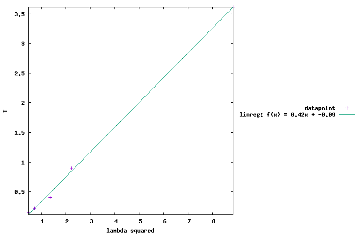
gnuplot is a tool for drawing 2 and 3 dimensional plots. You can either specify a function to plot, or you can simply read in data points from a file. I usually do the latter. Gnuplot also has a handy feature which allows one to perform a linear regression on a set of data points.

Below is the source code for a simple gnuplot (.gp) file which graphs a frequency with respect to tension from one of my lab reports. Note the text using 1:2 comes up several times. This tells gnuplot that the first column is the x axis and that the right column is the y axis. It is not necessary to use the first and second column for this purpose, but I find it more convenient. This gnuplot file also performs a linear regression on the data and displays that as well.

########10########20########30## DOCUMENTATION #50########60########70########80
#
#  OVERVIEW
#  ========
#  This gnuplot script will plot the left column of the input file as the x
#  axis, and the right column as the y axis. It will also perform a linreg on
#  the two.
#
#  The output file will be an EPS file named by appending .tex to the end of
#  ``filename``.
#
#  USAGE
#  =====
#
#  gnuplot -e "filename='somefile.csv'" plot.gp
#
########10########20########30##### LICENSE ####50########60########70########80
# Copyright (c) 2016, Charles Daniels
# All rights reserved.
#
# Redistribution and use in source and binary forms, with or without
# modification, are permitted provided that the following conditions are met:
#
# 1. Redistributions of source code must retain the above copyright notice,
# this list of conditions and the following disclaimer.
#
# 2. Redistributions in binary form must reproduce the above copyright notice,
# this list of conditions and the following disclaimer in the documentation
# and/or other materials provided with the distribution.
#
# 3. Neither the name of the copyright holder nor the names of its
# contributors may be used to endorse or promote products derived from this
# software without specific prior written permission.
#
# THIS SOFTWARE IS PROVIDED BY THE COPYRIGHT HOLDERS AND CONTRIBUTORS "AS IS"
# AND ANY EXPRESS OR IMPLIED WARRANTIES, INCLUDING, BUT NOT LIMITED TO, THE
# IMPLIED WARRANTIES OF MERCHANTABILITY AND FITNESS FOR A PARTICULAR PURPOSE
# ARE DISCLAIMED. IN NO EVENT SHALL THE COPYRIGHT HOLDER OR CONTRIBUTORS BE
# LIABLE FOR ANY DIRECT, INDIRECT, INCIDENTAL, SPECIAL, EXEMPLARY, OR
# CONSEQUENTIAL DAMAGES (INCLUDING, BUT NOT LIMITED TO, PROCUREMENT OF
# SUBSTITUTE GOODS OR SERVICES; LOSS OF USE, DATA, OR PROFITS; OR BUSINESS
# INTERRUPTION) HOWEVER CAUSED AND ON ANY THEORY OF LIABILITY, WHETHER IN
# CONTRACT, STRICT LIABILITY, OR TORT (INCLUDING NEGLIGENCE OR OTHERWISE)
# ARISING IN ANY WAY OUT OF THE USE OF THIS SOFTWARE, EVEN IF ADVISED OF THE
# POSSIBILITY OF SUCH DAMAGE.
########10########20########30########40########50########60########70########80

set datafile separator ","
set autoscale fix
set key outside right center
set terminal png medium size 740,480
set output sprintf("%s%s", filename, ".png")

set xlabel "lambda squared"
set ylabel "T"


f(x) = m*x + b
fit f(x) filename using 1:2 via m,b
title_f(a,b) = sprintf('linreg: f(x) = %.2fx + %.2f', m, b)

set title ""
plot filename using 1:2 with points title 'datapoint', f(x) title title_f(m,b)

Here is the output from this file:

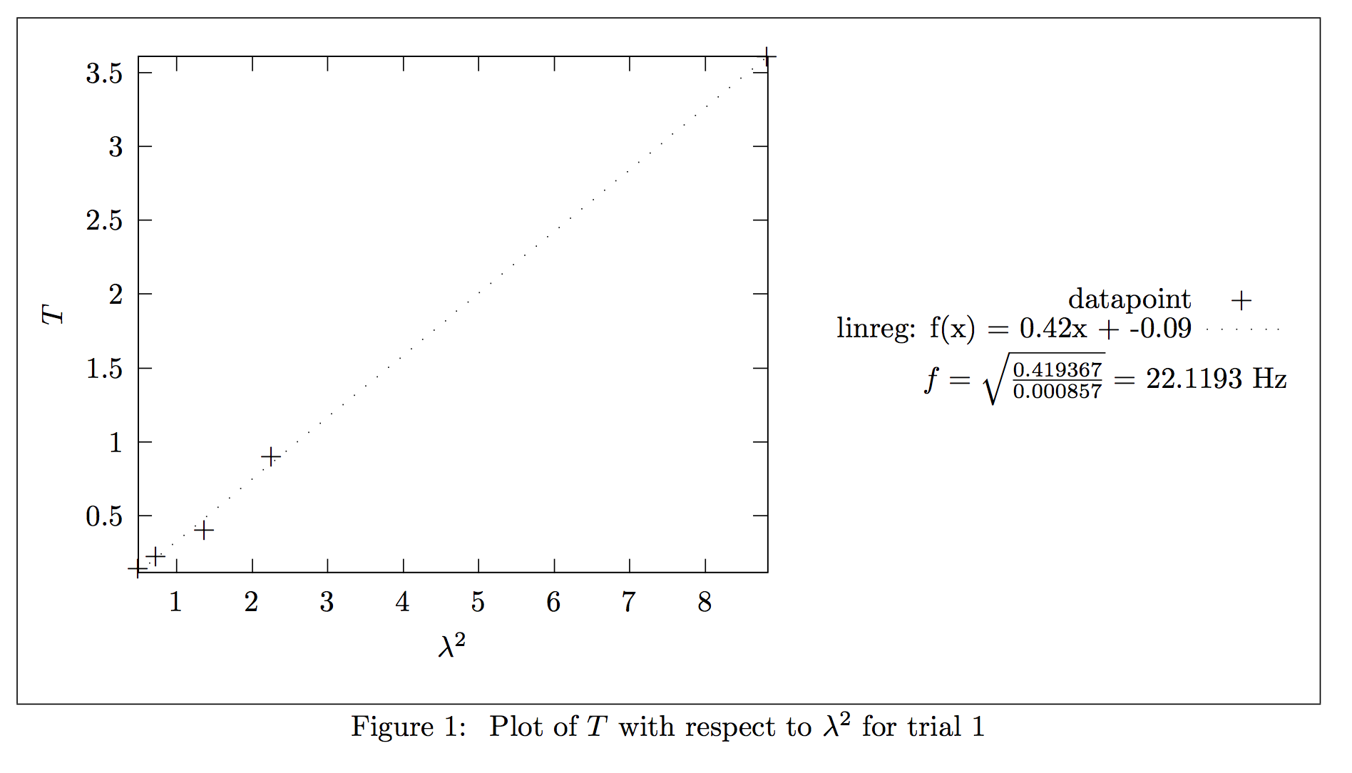
Note that as I usually do my reports in LaTeX, it is preferable to use a vector graphics format, rather than a raster format like png. To this end, gnuplot can be configured to emit EPS documents, which can then be included in a LaTeX document. I prefer to have gnuplot generate LaTeX (in the form of a .tex file) which renders the plot by simply using \input{plot.txt} in the document.

Here is the same gnuplot script, but modified to generate LaTeX:

########10########20########30## DOCUMENTATION #50########60########70########80
#
#  OVERVIEW
#  ========
#  This gnuplot script will plot the left column of the input file as the x
#  axis, and the right column as the y axis. It will also perform a linreg on
#  the two.
#
#
#  USAGE
#  =====
#
#  gnuplot -e "filename='somefile.csv'" plot.gp
#
########10########20########30#### LICENSE #####50########60########70########80
# Copyright (c) 2016, Charles Daniels
# All rights reserved.
#
# Redistribution and use in source and binary forms, with or without
# modification, are permitted provided that the following conditions are met:
#
# 1. Redistributions of source code must retain the above copyright notice,
# this list of conditions and the following disclaimer.
#
# 2. Redistributions in binary form must reproduce the above copyright notice,
# this list of conditions and the following disclaimer in the documentation
# and/or other materials provided with the distribution.
#
# 3. Neither the name of the copyright holder nor the names of its
# contributors may be used to endorse or promote products derived from this
# software without specific prior written permission.
#
# THIS SOFTWARE IS PROVIDED BY THE COPYRIGHT HOLDERS AND CONTRIBUTORS "AS IS"
# AND ANY EXPRESS OR IMPLIED WARRANTIES, INCLUDING, BUT NOT LIMITED TO, THE
# IMPLIED WARRANTIES OF MERCHANTABILITY AND FITNESS FOR A PARTICULAR PURPOSE
# ARE DISCLAIMED. IN NO EVENT SHALL THE COPYRIGHT HOLDER OR CONTRIBUTORS BE
# LIABLE FOR ANY DIRECT, INDIRECT, INCIDENTAL, SPECIAL, EXEMPLARY, OR
# CONSEQUENTIAL DAMAGES (INCLUDING, BUT NOT LIMITED TO, PROCUREMENT OF
# SUBSTITUTE GOODS OR SERVICES; LOSS OF USE, DATA, OR PROFITS; OR BUSINESS
# INTERRUPTION) HOWEVER CAUSED AND ON ANY THEORY OF LIABILITY, WHETHER IN
# CONTRACT, STRICT LIABILITY, OR TORT (INCLUDING NEGLIGENCE OR OTHERWISE)
# ARISING IN ANY WAY OUT OF THE USE OF THIS SOFTWARE, EVEN IF ADVISED OF THE
# POSSIBILITY OF SUCH DAMAGE.
########10########20########30########40########50########60########70########80

set datafile separator ","
set autoscale fix
set key outside right center

set terminal LaTeX size 6in,3in
set output sprintf("%s%s", filename ,'.tex')


set xlabel "$\\lambda^2$"
set ylabel "\\rotatebox{90}{$T$}"


f(x) = m*x + b
fit f(x) filename using 1:2 via m,b
title_f(a,b) = sprintf('linreg: f(x) = %.2fx + %.2f', m, b)

# calculate the frequency in Hz from the value of u that was passed in
freq = sqrt(m/u)
# this is an awful hack... absolute hardcoded positioning is bad
{% raw %} set label 1 sprintf("$f = \\sqrt{\\frac{%f}{%f}} = $ %3.4f Hz", m, u, freq) at screen 0.7, 0.45 # 12, 1.5 {% endraw %}

set title ""
plot filename using 1:2 with points title 'datapoint', f(x) title title_f(m,b)

This is what the compiled LaTeX output looks like:

Creating Figures with IPE

One challenge I encountered early on was producing nice-looking figures. Paint is nice, but it lack support for things like complex math equations and symbols. Paint also produces raster graphics, which bloats document size and don’t scale well.

I was recommended xfig by a professor (thanks Dr. Guiseppe!). I found that it produced nice results, although the interface was a little… dated.

The xfig User Interface

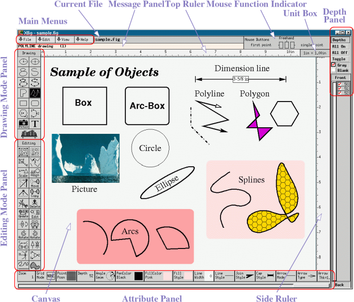
The xfig User Interface (image credit: mcj.sourceforge.net).

After some research, I came across somewhat of a spiritual successor to xfig: ipe. Ipe offers similar functionality, but with a native interface for macOS, Linux, and Windows, rather than using the now rather dated xlib GUI toolkit. Ipe also supports using LaTeX to generate labels with complex math symbols.

Here is an example of the ipe user interface while editing a figure from one of my lab reports:

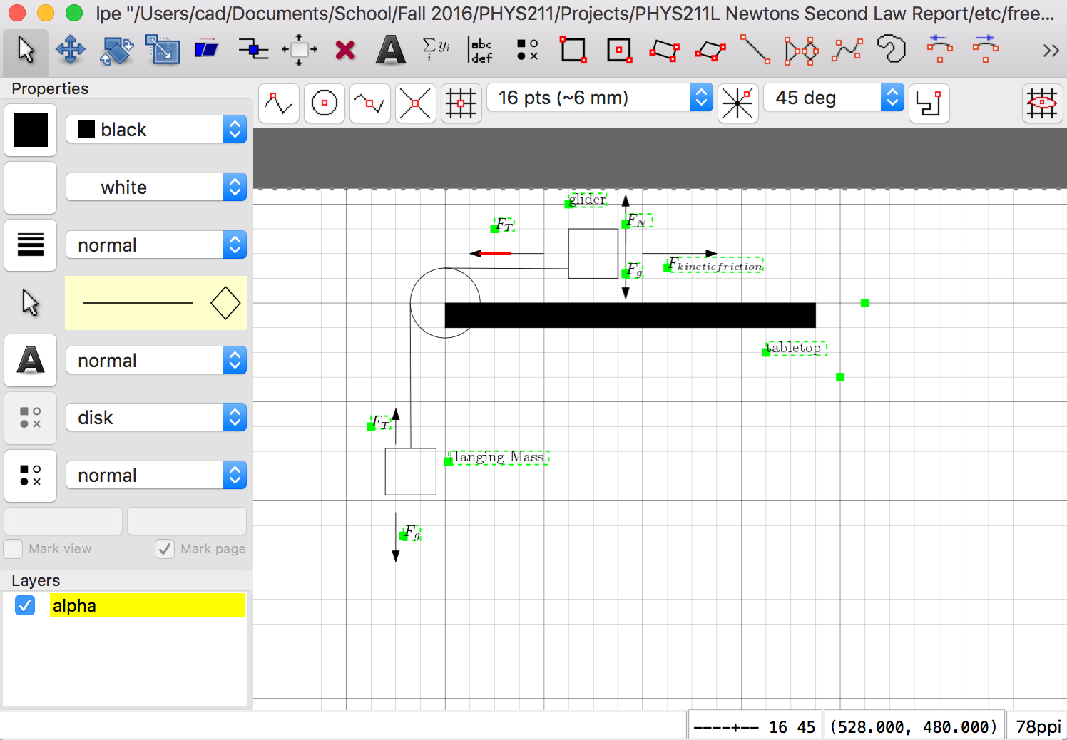
When a diagram is complete, ipe has an EPS-export feature, which produces a vector graphics rendering of your diagram, suitable for inclusion into the lab report. Even better, since ipe uses LaTeX to render labels, the fonts in the diagram will match the ones in the LaTeX document it is included in.

Creating Figures with PostScript

There are some rare cases when normal graphics packages like Paint, GIMP, or even ipe just won’t cut it. I ran into such a case when creating force table diagrams for a lab early on in the semester. In that case, I needed to draw accurately sized circles, arcs, and vectors. Trying to do this using gnuplot was impossible due to the way it handles polar plots. Doing it in a graphics package was also a nightmare - it’s very hard to draw an arc with precise angles without even a way to measure the arc being produced.

After discussing possible approaches to the problem with the professor, he encouraged me to try writing PostScript for my figures directly (again, thanks Dr. Guiseppe). This wound up producing excellent results.

For the uninformed, PostScript is the underlying technology used to render non-raster graphics in PDFs. PostScript is in effect, a programming language for drawing vector graphics. It is also the system used to print document from a computer - your computer’s printing system converts the document to be printed to PostScript, then sends that to the printer, which interprets, renders, and then prints it. It’s almost like gcode for printers.

The final PostScript code I came up with for these diagrams looked something like this:

%!PS-Adobe-3.0 EPSF-3.0
%%BoundingBox: 0 0 350 350
%%%%%%%10%%%%%%%%20%%%%%%%%30%%%%%%%%40%%%%%%%%50%%%%%%%%60%%%%%%%%70%%%%%%%%%80
% set up constants
/xcenter 175 def
/ycenter 175 def
/unitradius 100 def
/overshoot 50 def %how far past unit radius to draw axes and such
/offset 5 def  % small offsets, usually for labels
/arrowscale 1 def
/fontsize 8 def
%%%%%%%10%%%%%%%%20%%%%%%%%30%%%%%%%%40%%%%%%%%50%%%%%%%%60%%%%%%%%70%%%%%%%%%80
% symbol definitions
/s_deg (\312) def  % degree symbol, for some reason {\260} dosent seem to work
%%%%%%%10%%%%%%%%20%%%%%%%%30%%%%%%%%40%%%%%%%%50%%%%%%%%60%%%%%%%%70%%%%%%%%%80
% font setup
/Helvetica findfont  % font face
//fontsize scalefont setfont  % font size

% height of current font, from
% http://stackoverflow.com/questions/8296322/how-to-determine-height-and-depth-of-a-postscript-font
/fontheight currentfont dup /FontBBox get dup 3 get % top
  exch 1 get sub % top - bottom
  %␣adjusted␣by␣height␣multiplier/fontsize␣10␣def
  exch /FontMatrix get 3 get mul def
%%%%%%%10%%%%%%%%20%%%%%%%%30%%%%%%%%40%%%%%%%%50%%%%%%%%60%%%%%%%%70%%%%%%%%%80
% arrow head function
% found here:
% https://staff.science.uva.nl/a.j.p.heck/Courses/Mastercourse2005/tutorial.pdf

% draws an arrow head along the axis of the most recently drawn line. The
% first argument is the scale, the followign two are the x and y offsets.

{% raw %}/arrowhead {% stack: s x1 y1, current point: x0 y0 {% endraw %}
gsave
currentpoint % s x1 y1 x0 y0
4 2 roll exch % s x0 y0 y1 x1
4 -1 roll exch % s y0 y1 x0 x1
sub 3 1 roll % s x1-x2 y0 y1
sub exch % s y0-y1 x1-x2
atan rotate % rotate over arctan((y0-y1)/(x1-x2))
dup scale % scale by factor s
-7 2 rlineto 1 -2 rlineto -1 -2 rlineto
closepath fill % fill arrowhead
grestore
newpath
} def

%%%%%%%10%%%%%%%%20%%%%%%%%30%%%%%%%%40%%%%%%%%50%%%%%%%%60%%%%%%%%70%%%%%%%%%80

newpath
% draw the unit circle
//xcenter //ycenter //unitradius 0 360 arc
stroke
% draw the x and y axes
0.5 setlinewidth
//xcenter //ycenter moveto

//xcenter
//ycenter //unitradius add //overshoot add
lineto  % center to top

//xcenter
//ycenter //unitradius sub //overshoot sub
lineto  % center to bottom

//xcenter //ycenter moveto  % re-center cursor

//xcenter //unitradius add //overshoot add
//ycenter
lineto  % center to right

//xcenter //unitradius sub //overshoot sub
//ycenter
lineto  % center to left
stroke


%%%%%%%10%%%%%%%%20%%%%%%%%30%%%%%%%%40%%%%%%%%50%%%%%%%%60%%%%%%%%70%%%%%%%%%80↲
% draw labels

newpath
% move to the right outside of the unit circle, just above the x axis
//xcenter //unitradius add //offset add
//ycenter //offset add
moveto

(x) show

% move above the unit circle, just to the right of the y axis
//xcenter //offset add
//ycenter //unitradius add //offset add
moveto

(y) show

% draw the 0 deg vector
% first we draw the arrow head
newpath
//xcenter //ycenter translate
//unitradius //overshoot add 0 moveto
1 0 0 arrowhead
0 //xcenter sub 0 //ycenter sub translate
% now draw the 0 deg label itself
newpath

//xcenter //unitradius add //offset add
//ycenter //fontheight sub
moveto  % move to just below the x axis, right of the origin

(0) show //s_deg show

%%%%%%%10%%%%%%%%20%%%%%%%%30%%%%%%%%40%%%%%%%%50%%%%%%%%60%%%%%%%%70%%%%%%%%%80
% force table diagram for (13)

%%%%%%%10%%%%%%%%20%%%%%%%%30%%%%%%%%40%%%%%%%%50%%%%%%%%60%%%%%%%%70%%%%%%%%%80
% 145 deg arc
newpath
0 0 1 setrgbcolor  % set color

//xcenter //ycenter  % draw arc around the center
//unitradius 0.75 mul  % set the radius
0 60  % set the range in degrees for the first half of the arc
arc

(145) show //s_deg show  % arc label

//xcenter //ycenter
//unitradius 0.75 mul
60 145  % the range in degrees for the second half of the arc
arc

stroke

% reset color
0 0 0 setrgbcolor
%%%%%%%10%%%%%%%%20%%%%%%%%30%%%%%%%%40%%%%%%%%50%%%%%%%%60%%%%%%%%70%%%%%%%%%80

%%%%%%%10%%%%%%%%20%%%%%%%%30%%%%%%%%40%%%%%%%%50%%%%%%%%60%%%%%%%%70%%%%%%%%%80
% 227 deg arc
newpath
0 1 0 setrgbcolor  % set color

//xcenter //ycenter  % draw arc around the center
//unitradius 0.5 mul  % set the radius
0 60  % set the range in degrees for the first half of the arc
arc

(227) show //s_deg show  % arc label

//xcenter //ycenter
//unitradius 0.5 mul
60 227  % the range in degrees for the second half of the arc
arc

stroke

% reset color
0 0 0 setrgbcolor
%%%%%%%10%%%%%%%%20%%%%%%%%30%%%%%%%%40%%%%%%%%50%%%%%%%%60%%%%%%%%70%%%%%%%%%80

%%%%%%%10%%%%%%%%20%%%%%%%%30%%%%%%%%40%%%%%%%%50%%%%%%%%60%%%%%%%%70%%%%%%%%%80
% 31.4546 deg resultant vector arc
newpath
1 0 1 setrgbcolor  % set color

//xcenter //ycenter  % draw arc around the center
//unitradius 0.25 mul  % set the radius
0 15  % set the range in degrees for the first half of the arc
arc

(31.45) show //s_deg show  % arc label

//xcenter //ycenter
//unitradius 0.25 mul
15 31.4546  % the range in degrees for the second half of the arc
arc

stroke

% reset color
0 0 0 setrgbcolor
%%%%%%%10%%%%%%%%20%%%%%%%%30%%%%%%%%40%%%%%%%%50%%%%%%%%60%%%%%%%%70%%%%%%%%%80



%%%%%%%10%%%%%%%%20%%%%%%%%30%%%%%%%%40%%%%%%%%50%%%%%%%%60%%%%%%%%70%%%%%%%%%80
% 145 deg vector

% set color
0 0 1 setrgbcolor

% draw line
newpath
//xcenter //ycenter moveto
-102.394 71.6971  % x and y relative to origin of vector's end
rlineto

stroke

% used to ensure proper orientation for arrowheads
//xcenter //ycenter translate

-102.394 71.6971  % x and y relative to origin of vector's end
moveto  % move back to the end of the vector
1 0 0 arrowhead  % draw the arrowhead
stroke

-102.394 71.6971  % x and y relative to origin of vector's end
moveto  % move back to the end of the vector again so we can draw the label

(0.98N) show  % the actual label

0 0 0 setrgbcolor  % reset color
% turn translation back off, so 0 0 is the bottom left corner again
0 //xcenter sub
0 //ycenter sub
translate
%%%%%%%10%%%%%%%%20%%%%%%%%30%%%%%%%%40%%%%%%%%50%%%%%%%%60%%%%%%%%70%%%%%%%%%80

%%%%%%%10%%%%%%%%20%%%%%%%%30%%%%%%%%40%%%%%%%%50%%%%%%%%60%%%%%%%%70%%%%%%%%%80
% 227 deg vector

% set color
0 1 0 setrgbcolor

% draw line
newpath
//xcenter //ycenter moveto

-85.2498 -91.4192  % x and y relative to origin of vector's end
rlineto
stroke

% used to ensure proper orientation for arrowheads
//xcenter //ycenter translate

-85.2498 -91.4192  % x and y relative to origin of vector's end
moveto  % move back to the end of the vector
1 0 0 arrowhead  % draw the arrowhead
stroke

-85.2498 6 add -91.4192 % x and y relative to origin of vector's end
moveto  % move back to the end of the vector again so we can draw the label

(0.49N) show  % the actual label

0 0 0 setrgbcolor  % reset color
% turn translation back off, so 0 0 is the bottom left corner again
0 //xcenter sub
0 //ycenter sub
translate
%%%%%%%10%%%%%%%%20%%%%%%%%30%%%%%%%%40%%%%%%%%50%%%%%%%%60%%%%%%%%70%%%%%%%%%80

%%%%%%%10%%%%%%%%20%%%%%%%%30%%%%%%%%40%%%%%%%%50%%%%%%%%60%%%%%%%%70%%%%%%%%%80
% 0 deg vector

% set color
1 0 0 setrgbcolor

% draw line
newpath
//xcenter //ycenter moveto

125 0  % x and y relative to origin of vector's end
rlineto
stroke

% used to ensure proper orientation for arrowheads
//xcenter //ycenter translate

125 0 % x and y relative to origin of vector's end
moveto  % move back to the end of the vector
1 0 0 arrowhead  % draw the arrowhead
stroke

120 5  % x and y relative to origin of vector's end
moveto  % move back to the end of the vector again so we can draw the label

(1.47N) show  % the actual label

0 0 0 setrgbcolor  % reset color
% turn translation back off, so 0 0 is the bottom left corner again
0 //xcenter sub
0 //ycenter sub
translate
%%%%%%%10%%%%%%%%20%%%%%%%%30%%%%%%%%40%%%%%%%%50%%%%%%%%60%%%%%%%%70%%%%%%%%%80




%%%%%%%10%%%%%%%%20%%%%%%%%30%%%%%%%%40%%%%%%%%50%%%%%%%%60%%%%%%%%70%%%%%%%%%80
% Resultant vector (31deg)

% set color
1 0 1 setrgbcolor

% draw line
newpath
//xcenter //ycenter moveto

63.979 39.1367  % x and y relative to origin of vector's end
rlineto
stroke

% used to ensure proper orientation for arrowheads
//xcenter //ycenter translate

63.979 39.1367 % x and y relative to origin of vector's end
moveto  % move back to the end of the vector
1 0 0 arrowhead  % draw the arrowhead
stroke

63.979 39.1367  % x and y relative to origin of vector's end
moveto  % move back to the end of the vector again so we can draw the label

(0.39N) show  % the actual label

0 0 0 setrgbcolor  % reset color
% turn translation back off, so 0 0 is the bottom left corner again
0 //xcenter sub
0 //ycenter sub
translate
%%%%%%%10%%%%%%%%20%%%%%%%%30%%%%%%%%40%%%%%%%%50%%%%%%%%60%%%%%%%%70%%%%%%%%%80

This file, when rendered on a color computer screen, produces this image:

EDIT (2017-08-07): this image has been switched to JPEG format for browser compatibility. If you would like to view a high quality PDF format version, click this link.

As the above code is just a normal .eps file, it can be directly included in a LaTeX document to create a figure.

Processing Data with Python

I have experimented with several ways to process my input data to perform required calculations, and produce the content of my output data table.

I have experimented with several approaches to doing data processing automatically. I have settled finally on the idiomatic UNIX method: pipe the input data (sans headers) in on stdin, spew out the output data in CSV format on stdout. This allows easily using the resulting script as a part of a pipe, which make truncating or downsampling data easy when it is needed.

The actual contents of a typical Python script for processing this type of data is pretty straightforward. A few lines to read in the data, a few to print it out, and a bunch of equations in the middle. Here is an example from one of my labs:

#!/usr/local/bin/python3
########10########20########30## DOCUMENTATION #50########60########70########80
#
#  OVERVIEW
#  ========
#  Process data given on stdin. Output results to stdout
#
#  input lines are expected to be formatted as::
#
#    n,M,m,L,l
#
#  output lines are formatted as::
#
#    T,lmb2,lmb,d,n,V,u,f,L,l,m,M
#
#  NOTE: lmb stands for lambda
#
########10########20########30#### LISCENSE ####50########60########70########80
# Copyright (c) 2016, Charles Daniels
# All rights reserved.
#
# Redistribution and use in source and binary forms, with or without
# modification, are permitted provided that the following conditions are met:
#
# 1. Redistributions of source code must retain the above copyright notice,
# this list of conditions and the following disclaimer.
#
# 2. Redistributions in binary form must reproduce the above copyright notice,
# this list of conditions and the following disclaimer in the documentation
# and/or other materials provided with the distribution.
#
# 3. Neither the name of the copyright holder nor the names of its
# contributors may be used to endorse or promote products derived from this
# software without specific prior written permission.
#
# THIS SOFTWARE IS PROVIDED BY THE COPYRIGHT HOLDERS AND CONTRIBUTORS "AS IS"
# AND ANY EXPRESS OR IMPLIED WARRANTIES, INCLUDING, BUT NOT LIMITED TO, THE
# IMPLIED WARRANTIES OF MERCHANTABILITY AND FITNESS FOR A PARTICULAR PURPOSE
# ARE DISCLAIMED. IN NO EVENT SHALL THE COPYRIGHT HOLDER OR CONTRIBUTORS BE
# LIABLE FOR ANY DIRECT, INDIRECT, INCIDENTAL, SPECIAL, EXEMPLARY, OR
# CONSEQUENTIAL DAMAGES (INCLUDING, BUT NOT LIMITED TO, PROCUREMENT OF
# SUBSTITUTE GOODS OR SERVICES; LOSS OF USE, DATA, OR PROFITS; OR BUSINESS
# INTERRUPTION) HOWEVER CAUSED AND ON ANY THEORY OF LIABILITY, WHETHER IN
# CONTRACT, STRICT LIABILITY, OR TORT (INCLUDING NEGLIGENCE OR OTHERWISE)
# ARISING IN ANY WAY OUT OF THE USE OF THIS SOFTWARE, EVEN IF ADVISED OF THE
# POSSIBILITY OF SUCH DAMAGE.
########10########20########30########40########50########60########70########80

import sys
import csv
import numpy
import math
import logging

logging.basicConfig(level=logging.DEBUG)

output_format = ['T','lmb2','lmb','d','n','V','u','f','L','l','m','M']
precision = 3
g = 9.81  # gravity constant

logging.info("output format is: {}".format(','.join(output_format)))

for line in sys.stdin:
  line = line.replace('\\n', '')
  logging.debug("processing line: {}".format(line))
  line = [float(x) for x in line.split(',')]
  assert len(line) is 5
  n, M, m, L, l = line
  logging.debug("n, M, m, L, l = {}, {}, {}, {}, {}".format(n, M, m, L, l))

  # convert from grams to kg
  M *= 0.001
  m *= 0.001

  d = L/n
  T = M*g
  lmb = 2*d
  lmb2 = lmb * lmb
  u = m / l
  V = math.sqrt(T/u)
  f = V/lmb



  ns = locals()
  logging.debug("un-rounded output is: {}".format([ns[x] for x in output_format]))
  output = [str(round(ns[x], precision)) for x in output_format]
  logging.debug("generated output: {}".format(output))
  print(','.join(output))

I typically use a variation of this script, with the middle part changed to fit the bill for varying labs and data sets. This template is best suited for processing data where each input line corresponds to one output line (eg. no lookahead/lookback).

Also notice that I make use of the logging module. This is so I can easily display debugging information to stderr without clogging up my output on stdout. This makes things like ./script.py < input-data.csv > output- data.csv safe - only the CSV formatted rows are written to the output file.

Manipulating CSV Files with Command-Line Tools

I have found that CSV typically is the most pleasant format to use for storing and processing data. There are a plethora of UNIX tools which work very well with CSV files, and leveraging them allows for very powerful data manipulation.

Using `cut` to extract individual columns

In many cases, you have some data in a csv file that has many columns, but you only want certain ones. cut make it very easy to extract these.

Example

In this example, we have an input file c.csv, which has 7 columns. We only want the first, second, third, and fifth. Notice that cut supports mixing ranges and individual numbers in -f argument.

[cad@Daedalus.local][19:53:35][~/Desktop]
> cat c.csv
1,2,3,2,4,6,8
4,5,6,10,12,14,16
7,8,9,18,20,22,24
10,11,12,26,28,30,32
[cad@Daedalus.local][19:53:51][~/Desktop][130]
> cut -d, -f 1-3,5 < c.csv
1,2,3,4
4,5,6,12
7,8,9,20
10,11,12,28

Example

Here we extract only the 6th column from c.csv…

[cad@Daedalus.local][19:59:53][~/Desktop]
> cat c.csv
1,2,3,2,4,6,8
4,5,6,10,12,14,16
7,8,9,18,20,22,24
10,11,12,26,28,30,32
[cad@Daedalus.local][19:59:54][~/Desktop]
> cut -d, -f 6 < c.csv
6
14
22
30

Using `head` and `tale` to Truncate Data

In some cases, it may happen that you only want the first or last $n$ data points (lines) in a csv file. This is easy to accomplish with head and tail, which allow you to extract the first or last $n$ lines of a file respectively.

Example

Here, we show only the first 2 lines of c.csv…

[cad@Daedalus.local][19:56:52][~/Desktop]
> cat c.csv
1,2,3,2,4,6,8
4,5,6,10,12,14,16
7,8,9,18,20,22,24
10,11,12,26,28,30,32
[cad@Daedalus.local][19:56:57][~/Desktop]
> head -n 2 < c.csv
1,2,3,2,4,6,8
4,5,6,10,12,14,16

Example

Now the last 2 lines…

[cad@Daedalus.local][19:56:58][~/Desktop]
> cat c.csv
1,2,3,2,4,6,8
4,5,6,10,12,14,16
7,8,9,18,20,22,24
10,11,12,26,28,30,32
[cad@Daedalus.local][19:57:31][~/Desktop]
> tail -n 2 < c.csv
7,8,9,18,20,22,24
10,11,12,26,28,30,32

Example

Now the middle two…

> cat c.csv
1,2,3,2,4,6,8
4,5,6,10,12,14,16
7,8,9,18,20,22,24
10,11,12,26,28,30,32
[cad@Daedalus.local][19:58:25][~/Desktop]
> tail -n 3 < c.csv | head -n 2
4,5,6,10,12,14,16
7,8,9,18,20,22,24

Using `sed` to Downsample Data

Occasionally, we have some data which has been sampled at too high a rate. For example, imagine a sensor sampling at a rate of 200 datum per second. You are plotting the data with respect to time over a long period of time (eg. 1 hour). This would mean stuffing gnuplot with too many data points to handle. In this case, we could downsample the data to say 1 sample per second.

Fortunately, it is easy to make sed extract every $n^\text{th}$ line from a file, thus downsampling the data to $\frac{k}{n}$ datum per unit of time, where $k$ is the total number of datum.

Example In this example, we extract every other line ($n=2$) from d.csv. Note that on my system, GNU sed it gsed, as macOS ships BSD’s sed as the default.

[cad@Daedalus.local][21:14:04][~/Desktop]
> cat d.csv
1
2
3
4
5
6
7
8
9
10
11
12
13
14
15
16
17
18

[cad@Daedalus.local][21:14:05][~/Desktop]
> gsed -n "1p;0~2p" < d.csv
1
2
4
6
8
10
12
14
16
18

Using `paste` to move columns around

In some cases, you have several columns in different files, and you want to merge them into a single file. If this is the case, the paste command is the way to go.

Example

In this example, we have two files. One has three columns and one has four. We want to merge both together “side by side”.

[cad@Daedalus.local][19:43:47][~/Desktop]
> cat a.csv
1,2,3
4,5,6
7,8,9
10,11,12
[cad@Daedalus.local][19:43:49][~/Desktop]
> cat b.csv
2,4,6,8
10,12,14,16
18,20,22,24
26,28,30,32
[cad@Daedalus.local][19:43:50][~/Desktop]
> paste -d, a.csv b.csv
1,2,3,2,4,6,8
4,5,6,10,12,14,16
7,8,9,18,20,22,24
10,11,12,26,28,30,32

Example

I have found that sometimes, it is desirable to merge only specific columns. I’m sure there is a way to do this with paste along, but I find it easier to use cut in conjunction with paste. In this example, I merge column 2 of a.csv with column 3 of b.csv.

[cad@Daedalus.local][19:43:56][~/Desktop]
> cat a.csv
1,2,3
4,5,6
7,8,9
10,11,12
[cad@Daedalus.local][19:48:42][~/Desktop]
> cat b.csv
2,4,6,8
10,12,14,16
18,20,22,24
26,28,30,32
[cad@Daedalus.local][19:48:43][~/Desktop]
> cut -d, -f 2 < a.csv > a.col2.csv
[cad@Daedalus.local][19:48:59][~/Desktop]
> cut -d, -f 3 < b.csv > b.col3.csv
[cad@Daedalus.local][19:49:26][~/Desktop]
> paste -d, a.col2.csv b.col3.csv
2,6
5,14
8,22
11,30

When finished, the temporary files a.col2.csv and b.col3.csv can simply be deleted (eg. rm *.col*.csv).

Gluing it all Together with Make

All of these tools are great on their own, but what makes them shine is using them all together. I have found make to be the best way to accomplish this.

For the uninitiated, make is a tool for executing one or more commands, usually with the goal of building a binary or executable, while simultaneously resolving interdependencies between the command(s).

Example

Here is an example makefile from one of my lab reports.

Notice that, among other things, the data processing and plot generation are separate from producing the output PDF. This is because I often wish to only process the data or generate figures, without the whole report (usually for debugging).

Also notice in this case that I had to hardcore some variables, u_trial1, and u_trial2. This was to allow the calculated values of u to be displayed on the plot, which would have otherwise required excessive commandline gymnastics.

#TEXC=/usr/local/texlive/2016/bin/x86_64-linux/pdfLaTeX
TEXC=pdfLaTeX
TEXOPTS=--shell-escape
#BIBC=/usr/local/texlive/2016/bin/x86_64-linux/bibtex
BIBC=bibtex
BIBOPTS=
#MAKEINDEXC=/usr/local/texlive/2016/bin/x86_64-linux/makeindex
MAKEINDEXC=makeindex
MAKEINDEXOPTS=

# extracted from process_data logs to get around rounding issues
u_trial1=0.0008571428571428572
u_trial2=0.0003184713375796178

clean:
  -rm -rf out
  -rm -rf build

prep: clean
  -mkdir build
  -mkdir out
  cp -r src/* build
  cp -r etc/data/* build


data: prep
  cd build && ./process_data.py < data-trial1.csv > out-trial1.csv 2>out-trial1.log
  cd build && ./process_data.py < data-trial2.csv > out-trial2.csv 2>out-trial2.log
  -cp etc/*.eps build

plots: prep data
  cd build && gnuplot -e "filename='out-trial1.csv'" plot-png.gp 2> trial1-plot_png.log
  cd build && gnuplot -e "filename='out-trial2.csv'" plot-png.gp 2> trial2-plot_png.log
  cd build && gnuplot -e "filename='out-trial1.csv'; u=$(u_trial1)" plot-LaTeX.gp 2> trial1-plot_LaTeX.log
  cd build && gnuplot -e "filename='out-trial2.csv'; u=$(u_trial2)" plot-LaTeX.gp 2> trial2-plot_LaTeX.log

  mv build/out-trial1.csv.tex build/out-trial1-plot.tex
  mv build/out-trial2.csv.tex build/out-trial2-plot.tex



master: clean prep plots data
  cd build && $(TEXC) $(TEXOPTS) master
  cd build && $(BIBC) master

  cd build && $(TEXC) $(TEXOPTS) master
  cd build && $(TEXC) $(TEXOPTS) master

  cp build/*.pdf out/

Conclusion

This methodology and toolset has served me very well over the previous semester. While developing these tools and techniques required a considerable initial investment of time, writing lab reports is now a breeze - I just have to drop in the content, data, and equations and let the templates do the rest. Better yet, the whole thing can be stored in a revision control system like git.

2016-11-24

/posts/2016-11-24-lab-reports/ Charles Daniels

Target Audience

Workflow

LaTeX

Displaying CSV Files as Tables

Creating Plots With gnuplot

Creating Figures with IPE

Creating Figures with PostScript

Processing Data with Python

Manipulating CSV Files with Command-Line Tools

Using cut to extract individual columns

Using head and tale to Truncate Data

Using sed to Downsample Data

Using paste to move columns around

Gluing it all Together with Make

Conclusion

Using `cut` to extract individual columns

Using `head` and `tale` to Truncate Data

Using `sed` to Downsample Data

Using `paste` to move columns around